2026
Graph Neural Networks for Full Band-Structure Prediction in Architected Metamaterials
PosterMotivation
Designing a metamaterial for a target vibrational response is easier through inverse design. The problem is not bijective: many geometries give the same response, and testing each candidate by simulation is expensive. A design loop therefore needs two networks. A fast forward model that maps shape to response, and a generator that proposes shapes for a chosen response. Most deep learning work reduces the response to a bandgap width and a center frequency. This poster presents the forward model, which predicts the full band structure.
Forward model
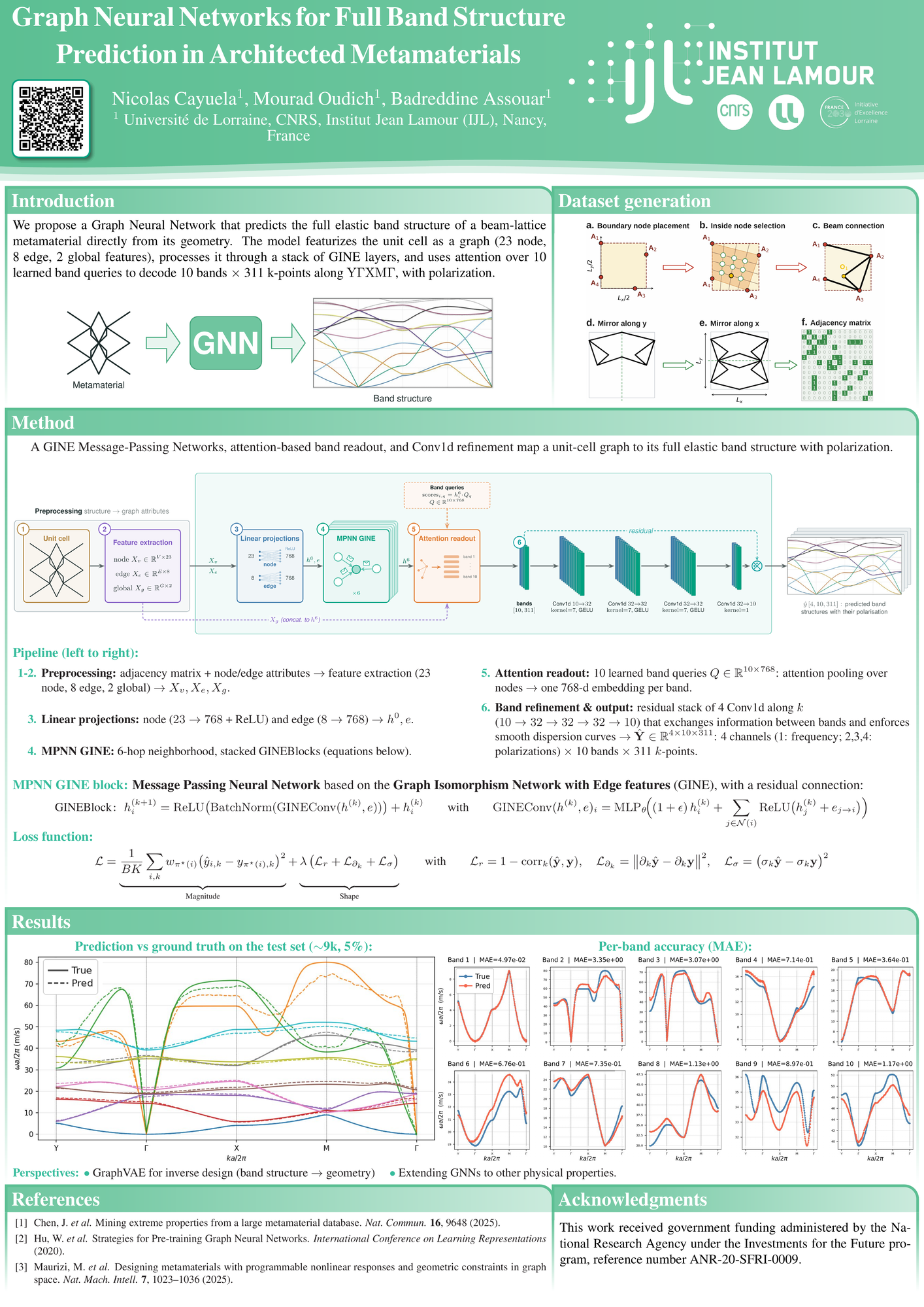
The model treats the unit cell as a graph. Junctions are the nodes, beams are the edges. Node and edge features are projected to dimension 768, then pass through six GINE message-passing layers. Each junction thus aggregates information up to about six nodes away. Ten learned band queries then aggregate the nodes by attention, one per band, and produce one vector per band. A short residual stack of 1D convolutions along the wavenumber axis mixes the bands and smooths the dispersion. The output is ten bands over 311 k-points along YΓXMΓ, each with a frequency and a polarization split over three channels (one longitudinal, two transverse).
$$h_i^{(l+1)} = \mathrm{ReLU}\!\big(\mathrm{BatchNorm}(\mathrm{GINEConv}(h^{(l)},e))\big) + h_i^{(l)}$$$$\mathrm{GINEConv}(h,e)_i = \mathrm{MLP}_\theta\!\Big((1{+}\epsilon)\,h_i + \!\!\sum_{j\in\mathcal{N}(i)}\!\! \mathrm{ReLU}(h_j + e_{j\to i})\Big)$$$$\alpha_{q,i} = \mathrm{softmax}_i\langle Q_q,\,h_i\rangle,\qquad z_q = \sum_i \alpha_{q,i}\,h_i$$$$\hat{y} = f_\theta(\mathcal{G})\in\mathbb{R}^{4\times 10\times 311}$$Training
Clean training data is the main difficulty: band labeling is not robust across geometries. To get around this, prediction and target are first matched optimally by a Hungarian assignment recomputed at every step, and the error is measured only afterward. The model is scored on the bands it finds, regardless of the order it lists them in. A few auxiliary terms on correlation, slope, and amplitude along k keep the upper bands from flattening. A second head predicts the polarization on the same matching.
$$\pi^\star = \arg\min_{\pi\in S_{10}} \sum_{j} \big\lVert \hat{y}_j - y_{\pi(j)}\big\rVert^2$$$$\mathcal{L} = \underbrace{\frac{1}{BK}\sum_{i,k} w_{\pi^\star(i)}\big(\hat{y}_{i,k} - y_{\pi^\star(i),k}\big)^2}_{\text{Magnitude}} + \lambda\,\underbrace{\big(\mathcal{L}_r + \mathcal{L}_{\partial_k} + \mathcal{L}_\sigma\big)}_{\text{Shape}}$$$$\mathcal{L}_r = 1 - \mathrm{corr}_k(\hat{\mathbf{y}},\mathbf{y}),\quad \mathcal{L}_{\partial_k} = \big\lVert \partial_k\hat{\mathbf{y}} - \partial_k\mathbf{y}\big\rVert^2,\quad \mathcal{L}_\sigma = \big(\sigma_k\hat{\mathbf{y}} - \sigma_k\mathbf{y}\big)^2$$Next
The next step is inverse design. A graph VAE will run the reverse path, from a target band structure to a geometry, and the same recipe should transfer to other physical properties.
Glossary
• GNN / GINE: graph neural network; GINE is a message-passing layer that accounts for edges.
• Message-passing: each node updates itself by aggregating information from its neighbors.
• Attention / band query: learned vectors that weight and aggregate nodes into one embedding per band.
• Residual stack: layers fed back into their input, refining it instead of replacing it.
• Hungarian matching: optimal one-to-one matching of predicted and true bands, so the model is scored on the set of curves, not their order.
• Forward / inverse model: predicts the response from a geometry / generates a geometry for a target response.
• Graph VAE: generative model on graphs, here for inverse design.
Notation
• \(\hat{y}\): Prediction
• \(y\): Target
• \(\pi^\star\): Optimal band permutation
• \(B\): Batch size
• \(K\): k-points per band
• \(w_b\): Per-band weight
• \(\lambda\): Weight of the shape terms
• \(\partial_k\): Derivative along k
• \(\sigma_k\): Standard deviation along k
• \(\mathrm{corr}_k\): Correlation along k
• \(Q_q\): Band query
• \(\mathcal{N}(i)\): Neighbours of node \(i\)Motivation
Concevoir un métamatériau pour une réponse vibratoire visée est plus simple par inverse design. Le problème n'est pas bijectif : plusieurs géométries donnent la même réponse, et tester chaque candidate par simulation coûte cher. Une boucle de conception demande donc deux réseaux. Un forward rapide qui va de la forme à la réponse, et un générateur qui propose des formes pour une réponse choisie. La plupart des travaux en deep learning réduisent la réponse à une largeur de bandgap et une fréquence centrale. Ce poster présente le modèle forward, qui prédit la structure de bandes complète.
Modèle forward
Le modèle voit la cellule unitaire comme un graphe. Les jonctions sont les nodes, les poutres les edges. Les features de nœuds et d'arêtes sont projetées en dimension 768, puis traversent six couches de message-passing GINE. Chaque jonction agrège ainsi l'information jusqu'à environ six nœuds de distance. Dix band queries apprises agrègent ensuite les nœuds par attention, une par bande, et produisent un vecteur par bande. Un court residual stack de convolutions 1D le long de l'axe du nombre d'onde mélange les bandes et lisse la dispersion. On obtient dix bandes sur 311 k-points le long de YΓXMΓ, chacune avec une fréquence et une répartition de polarisation en trois canaux (un longitudinal, deux transverses).
$$h_i^{(l+1)} = \mathrm{ReLU}\!\big(\mathrm{BatchNorm}(\mathrm{GINEConv}(h^{(l)},e))\big) + h_i^{(l)}$$$$\mathrm{GINEConv}(h,e)_i = \mathrm{MLP}_\theta\!\Big((1{+}\epsilon)\,h_i + \!\!\sum_{j\in\mathcal{N}(i)}\!\! \mathrm{ReLU}(h_j + e_{j\to i})\Big)$$$$\alpha_{q,i} = \mathrm{softmax}_i\langle Q_q,\,h_i\rangle,\qquad z_q = \sum_i \alpha_{q,i}\,h_i$$$$\hat{y} = f_\theta(\mathcal{G})\in\mathbb{R}^{4\times 10\times 311}$$Entraînement
Obtenir des données propres est la principale difficulté : l'étiquetage des bandes n'est pas robuste d'une géométrie à l'autre. Pour contourner cela, prédiction et cible sont d'abord appariées de façon optimale par une Hungarian assignment recalculée à chaque pas, et l'erreur n'est mesurée qu'ensuite. Le modèle est noté sur les bandes qu'il trouve, quel que soit l'ordre dans lequel il les liste. Quelques termes auxiliaires sur la corrélation, la pente et l'amplitude le long de k empêchent les bandes hautes de s'aplatir. Une seconde head prédit la polarisation sur le même appariement.
$$\pi^\star = \arg\min_{\pi\in S_{10}} \sum_{j} \big\lVert \hat{y}_j - y_{\pi(j)}\big\rVert^2$$$$\mathcal{L} = \underbrace{\frac{1}{BK}\sum_{i,k} w_{\pi^\star(i)}\big(\hat{y}_{i,k} - y_{\pi^\star(i),k}\big)^2}_{\text{Magnitude}} + \lambda\,\underbrace{\big(\mathcal{L}_r + \mathcal{L}_{\partial_k} + \mathcal{L}_\sigma\big)}_{\text{Shape}}$$$$\mathcal{L}_r = 1 - \mathrm{corr}_k(\hat{\mathbf{y}},\mathbf{y}),\quad \mathcal{L}_{\partial_k} = \big\lVert \partial_k\hat{\mathbf{y}} - \partial_k\mathbf{y}\big\rVert^2,\quad \mathcal{L}_\sigma = \big(\sigma_k\hat{\mathbf{y}} - \sigma_k\mathbf{y}\big)^2$$Suite
L'étape suivante est l'inverse design. Un graph VAE fera le chemin inverse, d'une structure de bandes visée vers une géométrie, et la même recette devrait se transposer à d'autres propriétés physiques.
Glossaire
• GNN / GINE : réseau de neurones sur graphe ; GINE est une couche de message-passing tenant compte des edges.
• Message-passing : chaque nœud se met à jour en agrégeant l'information de ses voisins.
• Attention / band query : vecteurs appris qui pondèrent et agrègent les nœuds en un embedding par bande.
• Residual stack : couches réinjectées dans leur entrée, elles l'affinent au lieu de la remplacer.
• Hungarian matching : appariement optimal un-à-un des bandes prédites et vraies, le modèle est noté sur l'ensemble des courbes, pas sur leur ordre.
• Forward / inverse model : prédit la réponse depuis une géométrie / génère une géométrie pour une réponse visée.
• Graph VAE : modèle génératif sur graphes, ici pour l'inverse design.
Notation
• \(\hat{y}\) : Prédiction
• \(y\) : Cible
• \(\pi^\star\) : Permutation optimale des bandes
• \(B\) : Taille du batch
• \(K\) : k-points par bande
• \(w_b\) : Poids par bande
• \(\lambda\) : Poids des termes de forme
• \(\partial_k\) : Dérivée selon k
• \(\sigma_k\) : Écart-type selon k
• \(\mathrm{corr}_k\) : Corrélation selon k
• \(Q_q\) : Band query
• \(\mathcal{N}(i)\) : Voisins du node \(i\)
Graph Neural Networks for Full Band-Structure Prediction in Architected Metamaterials Poster
Motivation
Designing a metamaterial for a target vibrational response is easier through inverse design. The problem is not bijective: many geometries give the same response, and testing each candidate by simulation is expensive. A design loop therefore needs two networks. A fast forward model that maps shape to response, and a generator that proposes shapes for a chosen response. Most deep learning work reduces the response to a bandgap width and a center frequency. This poster presents the forward model, which predicts the full band structure.
Forward model
The model treats the unit cell as a graph. Junctions are the nodes, beams are the edges. Node and edge features are projected to dimension 768, then pass through six GINE message-passing layers. Each junction thus aggregates information up to about six nodes away. Ten learned band queries then aggregate the nodes by attention, one per band, and produce one vector per band. A short residual stack of 1D convolutions along the wavenumber axis mixes the bands and smooths the dispersion. The output is ten bands over 311 k-points along YΓXMΓ, each with a frequency and a polarization split over three channels (one longitudinal, two transverse).
$$h_i^{(l+1)} = \mathrm{ReLU}\!\big(\mathrm{BatchNorm}(\mathrm{GINEConv}(h^{(l)},e))\big) + h_i^{(l)}$$$$\mathrm{GINEConv}(h,e)_i = \mathrm{MLP}_\theta\!\Big((1{+}\epsilon)\,h_i + \!\!\sum_{j\in\mathcal{N}(i)}\!\! \mathrm{ReLU}(h_j + e_{j\to i})\Big)$$$$\alpha_{q,i} = \mathrm{softmax}_i\langle Q_q,\,h_i\rangle,\qquad z_q = \sum_i \alpha_{q,i}\,h_i$$$$\hat{y} = f_\theta(\mathcal{G})\in\mathbb{R}^{4\times 10\times 311}$$Training
Clean training data is the main difficulty: band labeling is not robust across geometries. To get around this, prediction and target are first matched optimally by a Hungarian assignment recomputed at every step, and the error is measured only afterward. The model is scored on the bands it finds, regardless of the order it lists them in. A few auxiliary terms on correlation, slope, and amplitude along k keep the upper bands from flattening. A second head predicts the polarization on the same matching.
$$\pi^\star = \arg\min_{\pi\in S_{10}} \sum_{j} \big\lVert \hat{y}_j - y_{\pi(j)}\big\rVert^2$$$$\mathcal{L} = \underbrace{\frac{1}{BK}\sum_{i,k} w_{\pi^\star(i)}\big(\hat{y}_{i,k} - y_{\pi^\star(i),k}\big)^2}_{\text{Magnitude}} + \lambda\,\underbrace{\big(\mathcal{L}_r + \mathcal{L}_{\partial_k} + \mathcal{L}_\sigma\big)}_{\text{Shape}}$$$$\mathcal{L}_r = 1 - \mathrm{corr}_k(\hat{\mathbf{y}},\mathbf{y}),\quad \mathcal{L}_{\partial_k} = \big\lVert \partial_k\hat{\mathbf{y}} - \partial_k\mathbf{y}\big\rVert^2,\quad \mathcal{L}_\sigma = \big(\sigma_k\hat{\mathbf{y}} - \sigma_k\mathbf{y}\big)^2$$Next
The next step is inverse design. A graph VAE will run the reverse path, from a target band structure to a geometry, and the same recipe should transfer to other physical properties.
Glossary
• GNN / GINE: graph neural network; GINE is a message-passing layer that accounts for edges.
• Message-passing: each node updates itself by aggregating information from its neighbors.
• Attention / band query: learned vectors that weight and aggregate nodes into one embedding per band.
• Residual stack: layers fed back into their input, refining it instead of replacing it.
• Hungarian matching: optimal one-to-one matching of predicted and true bands, so the model is scored on the set of curves, not their order.
• Forward / inverse model: predicts the response from a geometry / generates a geometry for a target response.
• Graph VAE: generative model on graphs, here for inverse design.
Notation
• \(\hat{y}\): Prediction
• \(y\): Target
• \(\pi^\star\): Optimal band permutation
• \(B\): Batch size
• \(K\): k-points per band
• \(w_b\): Per-band weight
• \(\lambda\): Weight of the shape terms
• \(\partial_k\): Derivative along k
• \(\sigma_k\): Standard deviation along k
• \(\mathrm{corr}_k\): Correlation along k
• \(Q_q\): Band query
• \(\mathcal{N}(i)\): Neighbours of node \(i\)Motivation
Concevoir un métamatériau pour une réponse vibratoire visée est plus simple par inverse design. Le problème n'est pas bijectif : plusieurs géométries donnent la même réponse, et tester chaque candidate par simulation coûte cher. Une boucle de conception demande donc deux réseaux. Un forward rapide qui va de la forme à la réponse, et un générateur qui propose des formes pour une réponse choisie. La plupart des travaux en deep learning réduisent la réponse à une largeur de bandgap et une fréquence centrale. Ce poster présente le modèle forward, qui prédit la structure de bandes complète.
Modèle forward
Le modèle voit la cellule unitaire comme un graphe. Les jonctions sont les nodes, les poutres les edges. Les features de nœuds et d'arêtes sont projetées en dimension 768, puis traversent six couches de message-passing GINE. Chaque jonction agrège ainsi l'information jusqu'à environ six nœuds de distance. Dix band queries apprises agrègent ensuite les nœuds par attention, une par bande, et produisent un vecteur par bande. Un court residual stack de convolutions 1D le long de l'axe du nombre d'onde mélange les bandes et lisse la dispersion. On obtient dix bandes sur 311 k-points le long de YΓXMΓ, chacune avec une fréquence et une répartition de polarisation en trois canaux (un longitudinal, deux transverses).
$$h_i^{(l+1)} = \mathrm{ReLU}\!\big(\mathrm{BatchNorm}(\mathrm{GINEConv}(h^{(l)},e))\big) + h_i^{(l)}$$$$\mathrm{GINEConv}(h,e)_i = \mathrm{MLP}_\theta\!\Big((1{+}\epsilon)\,h_i + \!\!\sum_{j\in\mathcal{N}(i)}\!\! \mathrm{ReLU}(h_j + e_{j\to i})\Big)$$$$\alpha_{q,i} = \mathrm{softmax}_i\langle Q_q,\,h_i\rangle,\qquad z_q = \sum_i \alpha_{q,i}\,h_i$$$$\hat{y} = f_\theta(\mathcal{G})\in\mathbb{R}^{4\times 10\times 311}$$Entraînement
Obtenir des données propres est la principale difficulté : l'étiquetage des bandes n'est pas robuste d'une géométrie à l'autre. Pour contourner cela, prédiction et cible sont d'abord appariées de façon optimale par une Hungarian assignment recalculée à chaque pas, et l'erreur n'est mesurée qu'ensuite. Le modèle est noté sur les bandes qu'il trouve, quel que soit l'ordre dans lequel il les liste. Quelques termes auxiliaires sur la corrélation, la pente et l'amplitude le long de k empêchent les bandes hautes de s'aplatir. Une seconde head prédit la polarisation sur le même appariement.
$$\pi^\star = \arg\min_{\pi\in S_{10}} \sum_{j} \big\lVert \hat{y}_j - y_{\pi(j)}\big\rVert^2$$$$\mathcal{L} = \underbrace{\frac{1}{BK}\sum_{i,k} w_{\pi^\star(i)}\big(\hat{y}_{i,k} - y_{\pi^\star(i),k}\big)^2}_{\text{Magnitude}} + \lambda\,\underbrace{\big(\mathcal{L}_r + \mathcal{L}_{\partial_k} + \mathcal{L}_\sigma\big)}_{\text{Shape}}$$$$\mathcal{L}_r = 1 - \mathrm{corr}_k(\hat{\mathbf{y}},\mathbf{y}),\quad \mathcal{L}_{\partial_k} = \big\lVert \partial_k\hat{\mathbf{y}} - \partial_k\mathbf{y}\big\rVert^2,\quad \mathcal{L}_\sigma = \big(\sigma_k\hat{\mathbf{y}} - \sigma_k\mathbf{y}\big)^2$$Suite
L'étape suivante est l'inverse design. Un graph VAE fera le chemin inverse, d'une structure de bandes visée vers une géométrie, et la même recette devrait se transposer à d'autres propriétés physiques.
Glossaire
• GNN / GINE : réseau de neurones sur graphe ; GINE est une couche de message-passing tenant compte des edges.
• Message-passing : chaque nœud se met à jour en agrégeant l'information de ses voisins.
• Attention / band query : vecteurs appris qui pondèrent et agrègent les nœuds en un embedding par bande.
• Residual stack : couches réinjectées dans leur entrée, elles l'affinent au lieu de la remplacer.
• Hungarian matching : appariement optimal un-à-un des bandes prédites et vraies, le modèle est noté sur l'ensemble des courbes, pas sur leur ordre.
• Forward / inverse model : prédit la réponse depuis une géométrie / génère une géométrie pour une réponse visée.
• Graph VAE : modèle génératif sur graphes, ici pour l'inverse design.
Notation
• \(\hat{y}\) : Prédiction
• \(y\) : Cible
• \(\pi^\star\) : Permutation optimale des bandes
• \(B\) : Taille du batch
• \(K\) : k-points par bande
• \(w_b\) : Poids par bande
• \(\lambda\) : Poids des termes de forme
• \(\partial_k\) : Dérivée selon k
• \(\sigma_k\) : Écart-type selon k
• \(\mathrm{corr}_k\) : Corrélation selon k
• \(Q_q\) : Band query
• \(\mathcal{N}(i)\) : Voisins du node \(i\)